From Brute Force to HNSW: How Vector Search Gets Fast

Barakaeli Lawuo, Aug 22, 2026

In February 2017 three researchers at Facebook AI Research reported a search over Deep1B, a set of one billion image descriptors. Using 4 GPUs, their system found the true nearest neighbor as its first answer for 45.17% of queries, at 0.0133 ms per query when queries were sent in batches of 10,000.¹ The paper that introduced Deep1B had reported about the same accuracy (0.45) at 20 ms per query on a single CPU thread. The FAISS authors point out that the hardware differs, but call GPU search "a game-changer in terms of speed achievable on a single machine."¹

The setup behind that number is worth reading slowly. Each vector went through a learned linear transform called OPQ that cut it to 80 dimensions, was compressed to a 20 byte code, and filed into one of $2^{18}$ buckets. The whole index took about 20 GB.¹ Each of those choices fixes a cost left by a simpler method. This post starts at the simplest method, exact search, and adds them back one at a time.

Embedding

A list of numbers that a model produces to represent an item such as an image or a passage of text. The FAISS paper describes these as usually real-valued vectors with 50 to more than 1,000 dimensions.¹

Nearest neighbor search

Given a query vector, find the $k$ stored vectors closest to it, usually by Euclidean (L2) distance or cosine similarity.¹

Approximate nearest neighbor (ANN)

A search that finds the true neighbors with high probability "only," in the words of the product quantization paper, instead of with probability 1, in exchange for being much faster.²

Recall

The share of true nearest neighbors that the search actually returns. R@1 is the fraction of queries whose true nearest neighbor comes back as the top result.^1,4

QPS

Queries per second, the speed measure used by ANN-Benchmarks.⁴

Exact search costs N times d for every query

A vector database stores embeddings so it can answer one question: which stored vectors sit closest to this query? The direct answer is to compute the distance from the query to every stored vector and keep the smallest few. The product quantization paper gives the cost of this exhaustive search as $O(nD)$ for $n$ vectors of dimension $D$.² The FAISS paper notes that the expensive part is the dot product between query and database vector. With many queries at once, that becomes one large matrix multiplication, which is the kind of data-parallel work GPUs are good at.¹

Here is my own arithmetic for Deep1B. Its vectors have 96 dimensions: they are GoogLeNet image features, reduced by PCA and normalized to unit length.⁵ One exact query means $10^9 \times 96 = 9.6 \times 10^{10}$ multiply-adds, about 96 billion. A text search system with 10 million chunks and 768-dimensional embeddings would need $10^7 \times 768 \approx 7.7 \times 10^9$ per query. It gets worse as the collection grows, because the cost rises in a straight line with $N$.

Measured numbers agree. The HNSW paper timed brute force on one CPU thread: 94 ms per query on 1 million 128-dimensional SIFT vectors and 60 ms on a 1 million vector slice of Deep1B.³ If that scales linearly, which is my assumption, a full billion would take about a minute per query. Memory is the second bill. The FAISS authors put Deep1B's raw vectors at 384 GB.¹ Neither the minute nor the 384 GB works for a live service, and that is the problem every idea below is trying to fix.

Inverted lists: only scan the cells near the query

The first fix is to stop visiting every vector. Jégou, Douze and Schmid borrowed the inverted file, a structure already used for large-scale image search. Run k-means on the data to get $k'$ centroids, called the coarse quantizer. File each database vector in the list that belongs to its nearest centroid. At query time, find the query's nearest centroid and scan only that list.²

There is an obvious flaw: a query and its true neighbor often fall into different but adjacent cells. So the query is assigned to its $w$ nearest centroids, and all $w$ lists are scanned. The paper calls this multiple assignment. If the lists are roughly balanced, a query parses about $n \times w / k'$ entries, plus the $k'$ distance computations needed to pick the lists.² FAISS calls $w$ the multi-probe parameter $\tau$ and typically sets the number of lists near $\sqrt{N}$.¹ In my arithmetic, a billion vectors would then give about 31,600 lists, and probing 8 of them touches roughly 250,000 vectors instead of a billion.

Every neighbor outside the probed cells is simply gone. The paper is blunt about it: when $w$ is too small, the nearest neighbors not assigned to one of the $w$ centroids "are definitely lost," and no amount of extra precision in the stored vectors brings them back.² The index also still holds full vectors, so the 384 GB is untouched. Inverted lists cut compute and do nothing for memory.

Product quantization: store 8 bytes instead of 512

To shrink the vectors you can quantize them: replace each vector with the ID of its nearest centroid from a codebook. A 64-bit code would need $2^{64}$ centroids, far too many to learn or store.² Product quantization gets around this. It splits each $D$-dimensional vector into $m$ subvectors of $D/m$ dimensions and runs a small k-means with $k^*$ centroids on each part separately.² A vector's code is the list of $m$ centroid IDs. The combined codebook has $(k^*)^m$ centroids, but you only store $m \times k^*$ small ones. The paper calls $m = 8$ and $k^* = 256$ "often a reasonable choice": 8 bytes per vector.² A 128-dimensional float vector is 512 bytes, so that is 64 times smaller (my arithmetic).

The clever part is how distances are computed. The query is never compressed. Only the database vectors are. The paper calls this asymmetric distance computation (ADC):²

Here $x$ is the query at full precision, and $y$ is a stored vector known only by its code. $u_j(\cdot)$ takes the $j$th slice of a vector. $q_j$ is the $j$th sub-quantizer, which maps a slice of $y$ to one of its $k^*$ centroids. $d$ is Euclidean distance. For each query you compute, once, the squared distance from each query slice to all $k^*$ centroids of that slice. With $m = 8$ and $k^* = 256$, that is a table of 2,048 numbers (my count). After that, estimating the distance to any stored vector takes $m$ table lookups and additions, with no multiplications.²

Not compressing the query pays off. The authors prove that the expected squared error of the ADC estimate is bounded by the quantizer's mean squared error. If the query is compressed too, the bound is twice that.² In practice, with $m = 8$, ADC using 64 centroids per slice matched the accuracy of the symmetric method using 256.² The estimate is also biased low on average. The paper derives a correction, but finds it made neighbor search worse and recommends leaving it out unless you need the distance values themselves.²

Put the two ideas together and you get IVFADC. The inverted lists pick which cells to visit. Each list entry holds a vector ID plus a PQ code of the residual, the difference between the vector and its cell's centroid. Residuals are small, so they compress more accurately than the raw vectors would.² FAISS adds a practical note: IDs take 4 or 8 bytes, so a PQ code shorter than the ID gains nothing.¹ This is the structure behind the opening result.

What the lists and the codes buy, measured on GIST

The PQ paper's Table V puts real timings on this. The dataset is about one million 960-dimensional GIST image descriptors, queried 500 times with 64-bit codes. The quality measure is recall@100, the fraction of queries whose true nearest neighbor ranks somewhere in the top 100.²

Scanning every code with ADC took 17.2 ms and reached 0.652. IVFADC with 1,024 lists and 8 probes compared only 27,818 codes instead of 1,000,991, finished in 8.8 ms, and reached 0.682, beating the full scan on both speed and recall.² The authors explain why it can be more accurate as well as faster: coding the residual is more precise than coding the vector itself.² The chart also shows the tuning trap. With one probe, recall drops to 0.308 or 0.240. With 64 probes it climbs to 0.744, but the search takes 65.9 ms.²

The 8,192-list rows have lower recall than the 1,024-list rows at every $w$, and they are no faster. Their cells are smaller, so the same number of probes compares fewer codes: 361 instead of 1,947 at one probe.² The paper also warns that on small datasets the coarse quantizer itself can become the bottleneck, when $k' \times D$ exceeds $n/k'$.² My reading is that this is where the time went. Matching a 960-dimensional query against 8,192 centroids is about 7.9 million multiply-adds, far more than the list scan. The same paper's SIFT experiments found that for a fixed fraction of the data visited, more lists gave higher accuracy.² Which way it goes depends on the size of the dataset.

Memory is where PQ earns its place. On one million SIFT vectors, the IVFADC index took under 25 MB, while FLANN, a tree-based library that re-ranks with full vectors, needed more than 250 MB.² PQ was tested on a set of two billion SIFT vectors.² In the opening Deep1B run, 20 byte codes fit a billion vectors in about 20 GB, compared with 384 GB as raw floats.¹

HNSW: a skip list built from graphs

IVFADC leaves two costs: vectors lost at cell borders, and the accuracy ceiling set by the codes. Graph methods take a different route. Store each vector as a node and link it to nearby nodes. To search, start somewhere, keep moving to whichever neighbor is closest to the query, and stop when no neighbor is closer.³ Malkov and Yashunin note that on plain nearest-neighbor graphs, the number of steps grows as a power of the dataset size, and clustered data can split the graph into disconnected parts. Their earlier Navigable Small World (NSW) graphs improved this to polylogarithmic growth, but still slowed badly on low-dimensional data.³

Hierarchical NSW (HNSW) separates links by length into layers. When a node is inserted, it gets a random top layer $l = \lfloor -\ln(\mathrm{unif}(0,1)) \cdot m_L \rfloor$, so each layer up holds exponentially fewer nodes.³ A search starts at a fixed entry point in the top layer, where the few nodes are joined by long links. It walks greedily until it hits a local minimum, drops to the next layer from that node, and repeats. At layer 0, which holds every node, it keeps a candidate list of size $ef$, and $ef$ is the knob that trades speed for recall.³ The authors describe it as a probabilistic skip list with the linked lists replaced by proximity graphs, and recommend $m_L = 1/\ln(M)$, which matches a skip list with $p = 1/M$.³

Two more design choices matter. New links come from a heuristic, not simply the $M$ closest nodes: a candidate is linked only if it is closer to the new node than to any node already linked. This keeps links pointing in different directions and keeps separate clusters connected.³ And layer 0 allows up to $M_{max0} = 2M$ links per node. The paper suggests $M$ between 5 and 48, larger for high recall and high-dimensional data.³ Under the assumption of exact Delaunay graphs, the authors show the expected number of steps per layer is bounded by a constant. Since the number of layers grows as $O(\log N)$, so does search cost.³

Where the benchmark put each approach

ANN-Benchmarks, by Aumüller, Bernhardsson and Faithfull, runs every library in its own Docker container on one CPU thread, with a five-hour limit per setting, on Amazon c5.4xlarge machines. Each library is tested across many parameter settings, which traces out its curve of recall against QPS.⁴ Two of its datasets are GLOVE (1,183,514 word vectors, 100 dimensions, cosine similarity) and SIFT (1,000,000 vectors, 128 dimensions, Euclidean distance), each with 10,000 queries.⁴

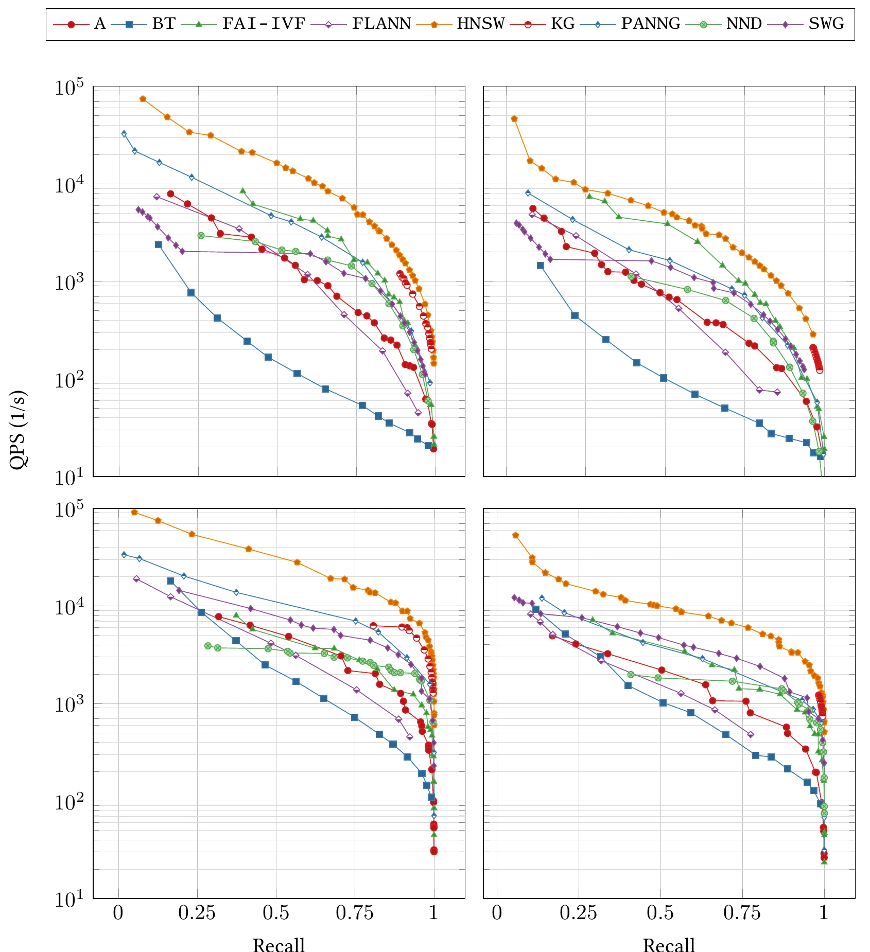
On GLOVE, HNSW was the fastest at every recall level, closely matched by KGraph (another graph method) at high recall, with FAISS-IVF third.⁴ On SIFT, all the methods could get close to perfect recall, and the graph methods were fastest.⁴ Note the vertical axis. It is logarithmic, and most curves drop by an order of magnitude or more over the last stretch toward recall 1. The authors observe that all the algorithms take a performance hit at high recall, with HNSW hit least.⁴

Batching changes the ranking. On a GPU with batched queries, FAISS's inverted file index answered about 655,000 queries per second at recall 0.7 and 61,000 at 0.99 on SIFT, 20 to 30 times its CPU speed. FAISS brute force on the same GPU managed about 24,000 queries per second.⁴ At a million vectors, then, exact search on a GPU is a realistic option. The index structures matter more as $N$ grows toward the billions in the opening.

What the graph costs: memory, rebuilds, and dimension

HNSW gets its speed by keeping full vectors plus a graph in RAM. The paper puts the link storage alone at about 60 to 450 bytes per object, not counting the data.³ With $M = 16$, $M_{max0} = 32$, and upper layers capped at $M$ links (my assumption), the formula $(M_{max0} + m_L M_{max})$ times 4 bytes gives about 150 bytes per vector. At a billion vectors, that is roughly 150 GB of links before any vector is stored (my arithmetic). In the paper's own comparison on 200 million SIFT vectors, HNSW peaked at 64 GB of RAM, against 30 GB and 23.5 GB for two FAISS PQ configurations. HNSW built faster, 42 minutes to 5.6 hours against 11 to 12 hours, and searched with much higher accuracy, but in the authors' words it "requires significantly more RAM."³

Changing data is the second weak spot. On GLOVE, the fastest HNSW index to reach recall 0.9 took almost 5 hours to build with the NMSlib implementation (FAISS's own HNSW did it in 1,700 seconds), against about 2 seconds for FAISS-IVF. The ANN-Benchmarks authors conclude that graph methods "might not be the preferred choice if the dataset changes regularly."⁴ HNSW does support incremental insertion, but its paper lists support for element updates and removal as future work.³ On the benchmark's Rand-Euclidean dataset, built so that each query's neighbors are easy to find locally but hard to reach through the data's overall structure, no HNSW setting got above 0.86 recall.⁴

The logarithmic scaling result also comes with a caveat about dimension. The proof assumes each node's number of neighbors in the Delaunay graph stays bounded, but that number grows exponentially with dimension. Checking the assumption empirically at $d = 128$ would take extremely large datasets, so the authors say more analytical evidence is needed to know whether it holds in high dimensions.³ Their own 200 million vector SIFT run showed query time growing faster than a pure logarithm, which they attribute, possibly, to the data's relatively high dimensionality.³ Embeddings, which the FAISS paper puts at 50 to more than 1,000 dimensions,¹ can sit far above the 128 of that test.