Test-time compute: the curve, the verifier, and the bill

Barakaeli Lawuo, Apr 29, 2026

In 2024 a team from Stanford, Oxford and Google DeepMind gave DeepSeek-Coder-V2-Instruct a set of real GitHub issues from SWE-bench Lite and let it try each one many times. With one attempt it solved 15.9% of them. With 250 independent attempts, at least one attempt solved the issue for 56% of them.¹ The best single-attempt system at the time, CodeStory Aide running a mix of GPT-4o and Claude 3.5 Sonnet, was at 43%.¹ The model had not changed. Each "attempt" was a full multi-turn session in the Moatless Tools agent framework, and the repository's own unit tests said whether it worked.¹

The same paper priced it. Five attempts per issue with DeepSeek solved 29.62% of issues for $10.80 in total, while one attempt each with GPT-4o solved 24.00% for $39 and Claude 3.5 Sonnet solved 26.70% for $51.¹ That is the case for test-time compute in one table: spending more computation when the model answers, instead of on a bigger model, and sometimes coming out ahead on both quality and price. The rest of this post follows the curve behind that result, the problem hidden inside it, and the measurements of when it stops paying.

Coverage is the number that climbs

Brown et al. split repeated sampling into two questions. Coverage asks: as the number of samples grows, what fraction of problems has at least one correct sample? Precision asks: can you actually find the correct sample among the others?¹ The 56% on SWE-bench Lite is coverage. It turned directly into solved issues only because unit tests can check every attempt automatically.¹

Test-time compute: computation spent while the model produces an answer: extra samples, search over partial solutions, or a longer reasoning trace.
Coverage (pass@k): the fraction of problems where at least one of k samples is correct. For code it is the same as the pass@k metric.
Verifier: whatever picks the final answer from the samples: unit tests, a proof checker, a majority vote, or a learned reward model.
Process reward model (PRM): a learned verifier that scores each intermediate step of a solution, not just the final answer.

Measuring pass@k by drawing exactly k samples is noisy, so both Brown et al. and the Codex paper before them draw a larger number N per problem, count the correct ones, and use an unbiased estimator.^1,2

\begin{aligned}\text{pass@}k &= \frac{1}{P}\sum_{i=1}^{P}\left(1-\frac{\binom{N-C_i}{k}}{\binom{N}{k}}\right)\end{aligned}

Equation 1 of Brown et al., following Chen et al.^1,2 P is the number of problems, N the samples drawn for each, and

C_i

how many of problem i's samples were correct. The fraction is the chance that k samples picked from the N contain none of the correct ones; one minus it is the chance of at least one hit.

The gains were not limited to one model or task. Across GSM8K, MATH, MiniF2F-MATH formal proofs, CodeContests and SWE-bench Lite, coverage rose smoothly as the budget grew to 10,000 samples per problem (250 for SWE-bench).¹ Gemma-2B went from 0.02% to 7.1% coverage on CodeContests. Pythia-160M went from 0.27% to 57% on MATH.¹ There was one clear exception: every Pythia model stayed at zero on CodeContests even at 10,000 samples, which the authors guess comes from Pythia seeing less code in training.¹ Sampling amplifies whatever probability the model already puts on a correct answer. If that probability is zero, more samples give you nothing.

The shape of the curve

Plotted against the log of the sample count, coverage often grows almost in a straight line over several orders of magnitude.¹ Brown et al. borrowed the function class the GPT-4 report used for training compute and fitted it to the log of coverage c as a function of the number of samples k.¹

\begin{gathered}\log c \approx a\,k^{b} \\ c \approx \exp\!\left(a\,k^{b}\right)\end{gathered}

Equations 2 and 3 of Brown et al.¹ a and b are fitted separately for each model and task.

Read it term by term. k is the number of independent samples per problem. b is negative in every fit the paper shows, so $k^{b}$ shrinks toward zero as k grows. a is also negative, so $a k^{b}$ is a negative number that rises toward zero, and c, its exponential, rises toward 1. At a single sample $k^{b} = 1$ , so $e^{a}$ is the curve's starting point (that follows from the algebra; it is not a separate claim in the paper). The size of b sets how quickly the curve climbs from there.

The fitted numbers make this concrete. For Llama-3-8B-Instruct on MATH, a is -1.33 and b is -0.43; on CodeContests, a is -3.88 and b is -0.11.¹ The math curve starts high and bends quickly toward full coverage. The code curve starts near 2% and climbs slowly. The measured data agree with the fit: on MATH, Llama-3-8B-Instruct reached 82.9% coverage at 100 samples and 98.44% at 10,000.¹

Computed from the fitted a and b values reported in Figure 5 of Brown et al., 2024,¹ not from their raw data points. The paper reports fit errors of 0.002 to 0.0056 for these three curves and warns that some curves, such as Llama-3-8B-Instruct on MiniF2F-MATH, do not follow the law closely.

The authors are careful about how far to trust this. The laws are "not as exact as training scaling laws," they write, and are best read as early evidence that inference scaling can be characterized.¹ They also found that models from the same family trace S-curves with similar slopes but different horizontal offsets. In practice that means the multiplicative increase in samples needed to move coverage from one level to another is roughly constant within a family.¹

Samples from a small model and samples from a large one cost different amounts, so the paper also redrew the curves against total inference FLOPs. At a fixed FLOP budget, Llama-3-8B-Instruct always beat the 70B model on coverage for MiniF2F, GSM8K and MATH. On CodeContests the 70B model was almost always the better buy.¹ Whether many cheap samples beat a few expensive ones depended on the task, and that question is where Snell et al. pick up.

Coverage is not accuracy

Coverage assumes a perfect verifier, one that always spots the correct sample if there is one. Math word problems have no unit tests, so Brown et al. tried three common substitutes on GSM8K and MATH: majority vote over final answers, best-of-N selection with the ArmoRM-Llama3-8B reward model, and a majority vote weighted by reward scores.¹ All three improved at first and then stopped improving at around 100 samples, while coverage kept rising past 95%.¹

Redrawn from numbers in Section 1 of Brown et al., 2024.¹ The gray bars are the largest gain any of the three selection methods achieved over this range. Coverage rose 15.5 points; the selectors gained under one.

For majority voting the reason is simple. Past a certain budget, the new correct answers are rare ones, and a rare answer cannot change which answer is most common.¹ Some problems had correct samples at rates of 1% or lower.¹ A verifier has to find the needle in a haystack of mostly wrong samples, and a vote is built to ignore needles.

The failure is not because the correct samples are lucky guesses. The authors hand-graded 105 chains of thought from correct Llama-3-8B-Instruct answers on GSM8K and found over 90% of them logically valid, even on problems where the model got 10% or fewer of its samples right.¹ The signal is there for a better verifier to use. Automatic verifiers are imperfect too: 11.3% of SWE-bench Lite problems had flaky tests that sometimes failed even the reference fix, and for 35 of the 122 CodeContests test problems with Python solutions, known correct solutions failed the provided tests.¹

One direction for better verifiers is the process reward model. Lightman et al. at OpenAI compared a reward model trained on final-answer correctness with one trained on human labels for each step. Picking the best of 1,860 samples on a representative subset of the MATH test set, the process-supervised model solved 78.2% of problems, against 72.4% for the outcome model and 69.6% for majority voting.³ Their training set, PRM800K, holds 800,000 step-level human labels.³

When extra inference beats a 14 times larger model

Snell et al., at UC Berkeley and Google DeepMind, asked the question an engineer with a fixed compute budget would ask: should the next FLOP go into a bigger model or into more inference?⁴ They worked on the MATH benchmark with PaLM 2-S*, fine-tuned for two ways of spending test-time compute. One was search against a PRM. The other was revisions, where the model rewrites its own previous answer in sequence.⁴ PRM800K did not work for them: a PRM trained on it was easy to exploit even with plain best-of-N, which they attribute to the gap between GPT-4 samples and PaLM 2 samples. So they trained their PRM without human labels, using per-step correctness estimates from Monte Carlo rollouts, the method of Wang et al.^4,5

Their central finding is that the best strategy depends on how hard the question is for the model. They measure difficulty as the model's own pass@1 rate, estimated from 2,048 samples and split into five equal-sized bins.⁴ On easy questions, beam search against the PRM got worse as the budget grew, a sign it was exploiting the verifier; on medium questions it beat best-of-N; on the hardest bin, "no method makes much meaningful progress."⁴ For revisions, easy questions did best with purely sequential compute, and harder ones with some mix of sequential and parallel.⁴ Choosing the strategy per difficulty bin, which they call compute-optimal scaling, matched or nearly matched best-of-N with up to 4 times less test-time compute.⁴

Then comes the exchange rate. Snell et al. approximate pretraining FLOPs as $X = 6ND_{\text{pretrain}}$ and inference FLOPs as $Y = 2ND_{\text{inference}}$ , where N is the parameter count and D a token count.⁴ Multiplying parameters by M multiplies both terms by M. To spend the same total on the small model instead, its inference compute can grow by this factor:⁴

\begin{gathered}M + 3\,\frac{D_{\text{pretrain}}}{D_{\text{inference}}}\,(M-1) \\ R = \frac{D_{\text{inference}}}{D_{\text{pretrain}}}\end{gathered}

The FLOPs-matching factor from Section 7 of Snell et al.⁴ The second term is the pretraining FLOPs the small model never spent, converted into extra inference tokens.

R is the whole story here. If a model will generate few tokens over its life compared with what it was trained on (R much less than 1), the pretraining savings buy a huge inference budget. If it will serve far more tokens than it saw in training, the savings spread thin. The paper tested R of 0.16, 0.79 and 22 against a model about 14 times larger decoding greedily.⁴ Plugging M = 14 into the formula is my arithmetic, not the paper's: the small model gets roughly 258 times its inference budget at R = 0.16, but only about 16 times at R = 22.

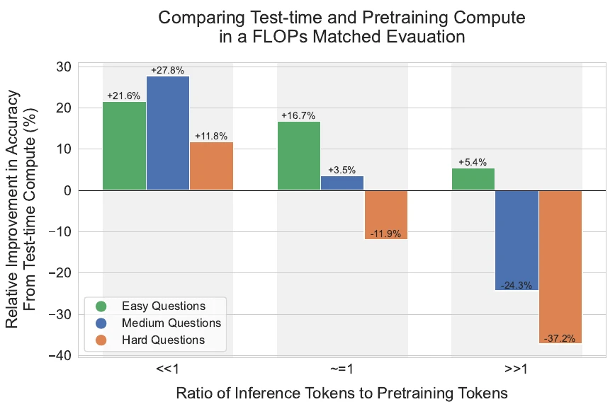
Grouped bar chart titled Comparing Test-time and Pretraining Compute in a FLOPs Matched Evaluation. Three groups by ratio of inference to pretraining tokens: much less than 1, about 1, much greater than 1. Each group has green, blue and orange bars for easy, medium and hard questions. At much less than 1 the bars are +21.6%, +27.8% and +11.8%. At about 1 they are +16.7%, +3.5% and -11.9%. At much greater than 1 they are +5.4%, -24.3% and -37.2%. — Top-right panel of Figure 1 (revisions) from Snell et al., 2024,⁴ reproduced under CC BY 4.0. Bars show the relative accuracy change from using test-time compute on PaLM 2-S* instead of a roughly 14 times larger model, at matched FLOPs. Above zero, test-time compute wins.

With revisions and a light inference load, test-time compute won in every difficulty group, by up to 27.8% on medium questions. At R much greater than 1 it still won on easy questions (+5.4%) but lost 24.3% on medium and 37.2% on hard ones.⁴ PRM search followed the same pattern and lost harder: -52.9% on hard questions at the heaviest inference load.⁴ The authors' summary is that test-time and pretraining compute are "not 1-to-1 exchangeable." Test-time compute can stand in for a bigger model on questions within the model's reach, or when inference volume is small. On questions beyond it, or at high volume, pretraining is likely the better buy.⁴ There is a cost the comparison leaves out: sorting a question into a difficulty bin itself takes a non-trivial amount of inference, and the experiments do not count it.⁴

Longer thinking, forced: s1's budget forcing

Everything so far spends compute in parallel, or in rounds of full answers. Muennighoff et al. went the other way and spent it inside a single, longer reasoning trace. They fine-tuned Qwen2.5-32B-Instruct on just 1,000 curated questions with reasoning traces distilled from Gemini Thinking. Training took 26 minutes on 16 H100 GPUs, and the result is s1-32B.⁶

Budget forcing controls how long it thinks. To cap the thinking, you append the end-of-thinking delimiter (and optionally "Final Answer:"), and the model moves straight to its answer. To make it think longer, you block the delimiter and append "Wait" instead.⁶ The paper's Figure 3 shows why this can work. Asked how many r's are in "raspberry," the model counts two and tries to stop; after the forced "Wait" it rereads the word, counts three, and notes that its first answer came from reading too quickly.⁶

Redrawn from Table 1 of Muennighoff et al., 2025.⁶ AIME24 has 30 problems, so each problem is worth 3.3 points and the 6.7 point gain from budget forcing is two problems (the author's arithmetic).

The paper scores a scaling method on three things: control (whether it stays within the requested budget), scaling (the average slope of accuracy against thinking tokens), and the best accuracy it reaches.⁶ On AIME24, budget forcing had 100% control, a slope of 15, and 56.7% accuracy. Telling the model a token limit in the prompt gave 40% control and a negative slope of -24, because the model cannot reliably count its own tokens.⁶ Rejection sampling, which resamples until an answer fits the length limit, had a slope of -35. Longer answers were more often wrong, which the authors think happens because long traces tend to be the ones where the model went off track and had to backtrack.⁶ The word "Wait" mattered too: ignoring the stop twice gave 53.3% on AIME24 with "Wait," but 50.0% with no string or with "Hmm" or "Alternatively."⁶ Majority voting over the base Qwen model's samples could not catch up with s1-32B.⁶

Where the curve flattens

Budget forcing does not scale without limit. Accuracy on AIME24 stopped improving by the sixth forced "Wait," and blocking the stop too often pushed the model into repetitive loops instead of more reasoning.⁶ The second limit is the context window. When the authors instead told the model in the prompt to use up to 512 reasoning steps, 12 of the 30 AIME24 questions produced responses longer than the context window, and performance dropped sharply.⁶ In the authors' own words, budget forcing "eventually flattens out," and "the context window of the underlying language model constrains it."⁶