Four serving metrics and the stalls they hide

Barakaeli Lawuo, Mar 11, 2026

In a paper posted in July 2024, a group from Georgia Tech, Microsoft Research India and Intel reported running two LLM serving systems, vLLM and Sarathi-Serve, on the same job: Yi-34B on two H100 GPUs, answering requests from an arXiv summarization trace at 1.5 queries per second. In vLLM, almost 60% of requests waited more than 25 seconds before the server even started on their prompt. In Sarathi-Serve, no request waited longer than 15 seconds. Yet the two systems' normalized latency, a standard number for comparing serving systems, differed by only a few hundred milliseconds.¹

The reason is arithmetic. Normalized latency divides a request's total time by the number of tokens it generated, and the median request in that trace generated 228 tokens, so a 25 second wait shrinks to about a tenth of a second per token (25 divided by 228).¹ The paper, first posted as Metron and renamed Etalon in its second version, goes through the usual serving metrics one by one and shows where each goes blind.¹ This post follows the same order. For each metric: the exact definition, how a benchmark measures it, and the case the metric misses.

Prefill: The first phase of a request, where the model reads the whole prompt and produces the first output token.
Decode: The second phase, where the model produces output tokens one at a time, each step feeding the last token back in.
Scheduling delay: Time a request spends waiting in the server's queue before its prompt processing starts.
SLO: Service level objective: a latency target the system promises to meet for some share of requests, such as 99%.
Tail latency: A high percentile of the latency distribution, such as the 99th, which describes the slowest requests rather than the typical one.

Time to first token adds a queue to a prompt

Time to first token (TTFT) is the gap between a request arriving and the system producing its first output token.¹ The Metron paper splits it into two parts:

\begin{gathered} \mathrm{TTFT} = t_{\text{first}} - t_{\text{arrive}} \\[4pt] = d_{\text{sched}} + T_{\text{prefill}}(P) \end{gathered}

TTFT as the sum of scheduling delay and prompt processing time, following the definition in Agrawal et al., 2024.¹

$t_{\text{arrive}}$ is when the request reaches the server and $t_{\text{first}}$ is when the first token comes out. $d_{\text{sched}}$ is the scheduling delay, which depends on load, routing and batching policy. $T_{\text{prefill}}(P)$ is the time to process a prompt of $P$ tokens.¹ A client measuring a hosted API sees one more term folded in: network time. The 2026 measurement study of hosted open-weight APIs by the AI Ping team defines TTFT as wall-clock time from request submission to the first streamed token, and notes that end-to-end latency is shaped by input length, output length, queuing, provider-side batching and network delay.³

The blind spot is that one number mixes two causes. Two systems with the same TTFT could have very different queues and very different prefill speeds, and TTFT alone does not say which.¹ It also grows with prompt length. Metron's Figure 1 shows prefill time for Yi-34B on two H100s rising steeply from 512 to 32K tokens, and the authors call the growth quadratic.¹ So a single fixed TTFT target makes little sense when prompts vary: in the LMSys-Chat-1M conversation dataset, which Metron cites, the median prompt is 417 tokens and the 90th percentile is 1,418.¹ Dividing TTFT by prompt length does not fix it either, because that also divides the queueing delay and so treats short prompts unfairly.¹

MLPerf Inference, the industry benchmark described by Reddi et al. in 2019, predates LLM streaming and has no first-token metric. It does show how a standard benchmark pins down a latency limit. In its server scenario, queries arrive at random following a Poisson process, and each task gets a fixed latency bound between 15 and 250 milliseconds. No more than 1% of queries may exceed it for vision tasks, and no more than 3% for translation.² Each server query there carries a single sample from an image or translation task. An LLM prompt can run from hundreds to thousands of tokens, and a bound that ignores that is the problem Metron raises about TTFT targets.

Time per output token averages away the stall

After the first token, two related metrics describe decode speed. Time between tokens (TBT) is the latency of each individual token after the first. Time per output token (TPOT) is the average: total decode time divided by the number of decode tokens.¹ DistServe, a 2024 serving paper, uses TTFT and TPOT as its two latency targets.⁴

\begin{gathered} \mathrm{TBT}_i = t_i - t_{i-1} \\[4pt] \mathrm{TPOT} = \frac{T_{\text{decode}}}{N_{\text{decode}}} \\[4pt] \mathrm{NormLat} = \frac{T_{\text{e2e}}}{N_{\text{decode}}} \end{gathered}

TBT, TPOT and normalized latency, following the definitions in Agrawal et al., 2024.¹

$t_i$ is when token $i$ reaches the user. $T_{\text{decode}}$ is the time from the first token to the last, $N_{\text{decode}}$ is the number of decode tokens, and $T_{\text{e2e}}$ is the full request time including queueing and prefill. Normalized latency is the metric from the opening, and the only difference from TPOT is that its numerator includes the queue.¹

Both averages hide stalls, and they do it the same way. In Metron's Figure 3a, a vLLM request stops producing tokens for about 10 seconds, which the authors say can happen when a long prefill from another request joins the running batch. For a reader that is a frozen screen. Spread over a long output, it barely moves TPOT or normalized latency.¹ The authors give a reading-speed reference point: at 250 words per minute, a reader needs roughly 6 tokens per second.¹ A system can beat that on average and still stop dead for ten seconds.

The obvious fix is to report tail TBT, say the 99th percentile, as the Sarathi-Serve paper did.^1,5 Metron shows that this goes wrong the other way. In one test with 1,000 requests, vLLM and Sarathi-Serve looked about the same on TPOT-based throughput. vLLM's tail TBT was much worse, about 1 second, yet vLLM had lower TBT than Sarathi-Serve between the 80th and 98th percentiles, and the two had comparable medians. In the paper's words, TPOT "downplays the discrepancies between the systems" while tail TBT "overstates them".¹ A TBT percentile also cannot say whether a stall hit the first token or the last, or how many stalls a single request suffered.¹

Speculative decoding breaks per-token timing in another way. That technique, from Leviathan et al., computes several tokens in parallel to speed up exact decoding.⁶ Suppose three tokens arrive together after time $T$ , then the next arrives after $3T$ . Counted token by token, the TBTs are $T$ , 0, 0 and $3T$ , and the $3T$ looks like a stall. But the user got 4 tokens in $4T$ , and a client could have shown them at an even pace.¹ When Metron measured public APIs, about 90% of decode tokens from Fireworks arrived together, which the authors read as a hint that it uses speculative decoding.¹

Throughput describes the server, not the reader

"Throughput" means two different things, and people mix them up. System throughput counts output tokens across all users: DistServe describes it as tokens generated per second across all users and requests.⁴ Per-request speed is the rate one user sees, often reported as the inverse of TPOT. The AI Ping study calls this tokens per second (TPS): output tokens divided by generation time after the first token.³

\begin{gathered} X_{\text{sys}} = \frac{\sum_r N_{\text{out}}(r)}{T_{\text{window}}} \\[4pt] \mathrm{TPS}_r = \frac{N_{\text{out}}(r)}{t_{\text{last}} - t_{\text{first}}} \end{gathered}

System throughput over a measurement window, and per-request TPS as defined by Li et al., 2026.^3,4

$X_{\text{sys}}$ sums the output tokens $N_{\text{out}}(r)$ of every request $r$ finished in a window of length $T_{\text{window}}$ . $\mathrm{TPS}_r$ divides one request's output tokens by its own generation time. Serving systems raise $X_{\text{sys}}$ by batching many requests, and bigger batches can slow each one down. That trade-off is why a throughput number means little without the latency it was measured at.

MLPerf builds this into its rules. Its offline scenario sends all samples at once with no latency limit and reports samples per second. Its server scenario reports the query rate a system can sustain while staying within the latency bound.² In the first round of results, every system delivered less throughput in the server scenario than offline, which the authors blame on the latency limit and the smaller batches it forces. Across the five systems with translation results, the drop was 39% to 55%. For ResNet-50 it ranged from 3% to 35%, averaging about 20%, and for MobileNet-v1 it averaged under 10%.² The authors conclude that a comparison with unconstrained latency "has little bearing on a latency-constrained scenario".²

Tail limits also cost measurement time. MLPerf sets the number of queries needed so the reported percentile holds with 99% confidence, using an error margin one-twentieth of the gap between the percentile and 100%.²

\begin{gathered} m = \frac{1 - p}{20} \\[4pt] N = \left(\Phi^{-1}\!\left(\tfrac{1-c}{2}\right)\right)^{2} \frac{p\,(1-p)}{m^{2}} \end{gathered}

Equations 1 and 2 of Reddi et al., 2019,² with

p

the tail-latency percentile,

c

the confidence level,

m

the margin and

\Phi^{-1}

the inverse standard normal CDF (NormsInv in the paper).

The margin shrinks as the percentile rises, and $N$ grows with $1/m^2$ , so tighter tails need far more queries. MLPerf rounds each count up to a multiple of $2^{13}$ .²

Redrawn from Table IV of Reddi et al., 2019.² Unrounded counts are 23,886, 50,425 and 262,742 at 99% confidence. By the same formula, a p99 taken from a few hundred requests carries a far wider margin.

For hosted APIs, per-request speed also depends on which provider serves the model and when. The AI Ping study used request logs and latency measurements collected by the AI Ping service from October to December 2025. It found listed prices clustered near official prices while TTFT and throughput varied widely across providers of the same model, and official endpoints were not always the fastest.³ Its Figure 10, below, compares throughput in the first and last week after each model was listed.

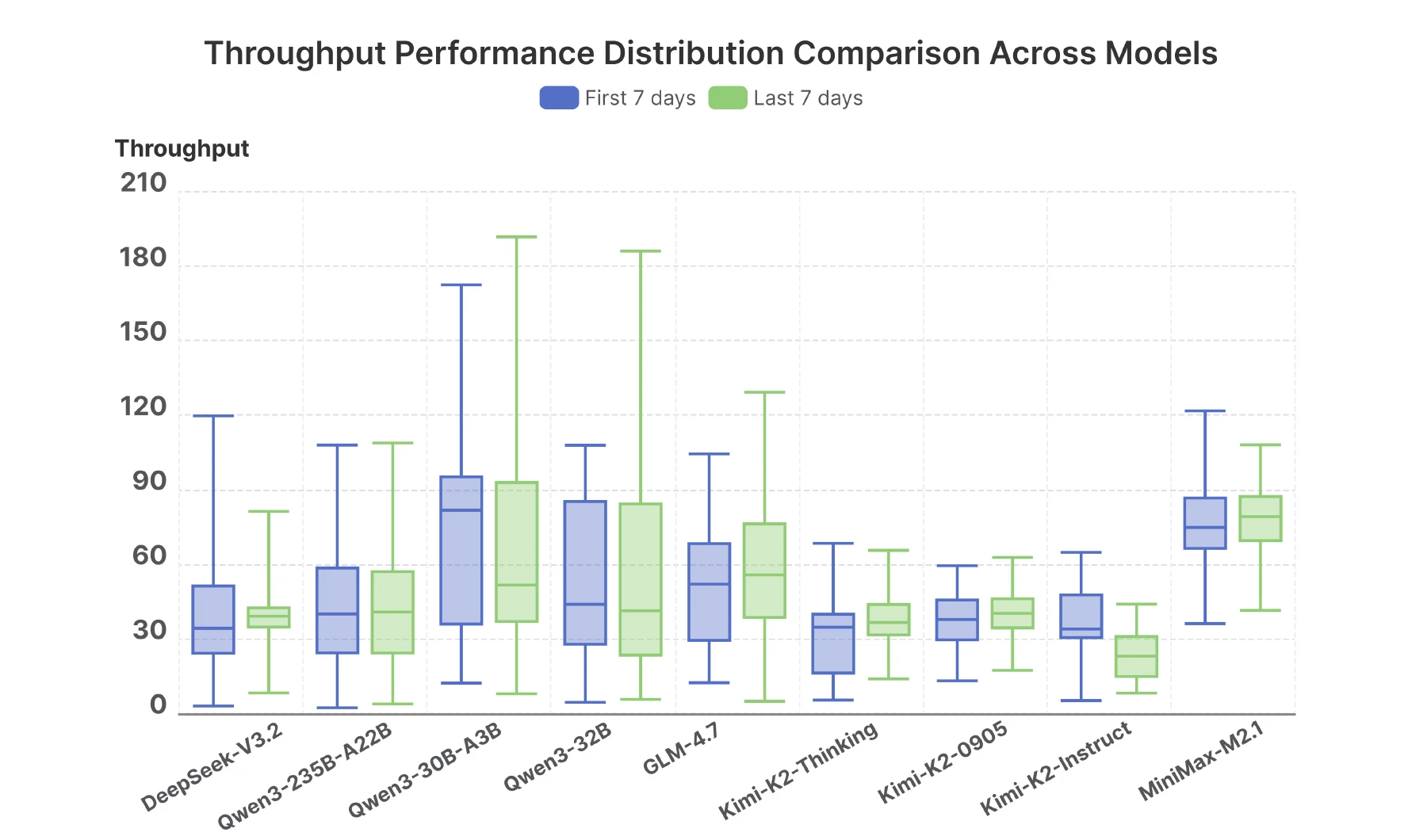
Box plots of throughput for nine hosted open-weight models, comparing the first seven days after listing with the last seven days of the measurement period. Boxes are wide and whiskers span from near zero to over 100 tokens per second for several models. — Figure 10 from Li et al., 2026,³ reproduced under CC BY 4.0. Each pair of boxes is one model's throughput distribution in the first and last observed week. The authors describe the figure as descriptive, not controlled for request length or task mix.

The spread inside a single box is the point. A published "tokens per second" for a model is one draw from a wide distribution, and the authors warn that a routing policy built on one historical measurement "can become stale".³ For DeepSeek-V3.2 they report that routing requests across providers raised average TPS by about 90% over calling the official endpoint directly, across about one million requests.³

Cost per million tokens inherits every throughput error

Cost per token is not measured directly. It is derived from a throughput figure and a price. For self-hosted serving, the arithmetic is mine but the structure is standard:

C_{\text{1M}} = \frac{G \cdot p_{\text{GPU}}}{3600 \cdot X_{\text{sys}}} \times 10^{6}

Cost per million output tokens for self-hosted serving. The author's arithmetic, not a formula from the cited papers.

$G$ is the number of GPUs, $p_{\text{GPU}}$ is the price of one GPU-hour, 3600 turns hours into seconds, and $X_{\text{sys}}$ is sustained system throughput in tokens per second. Everything that goes wrong with $X_{\text{sys}}$ goes wrong here too. If you take $X_{\text{sys}}$ from an offline run and then serve under a latency limit, MLPerf's translation results say throughput can fall 39% to 55%.² Because cost is inversely proportional to throughput, that makes the real cost per token $1/(1-0.39) \approx 1.6$ to $1/(1-0.55) \approx 2.2$ times the offline estimate. DistServe makes the same point from the other direction: it measures goodput, the request rate a GPU can serve while meeting the latency targets, because higher per-GPU goodput "directly translates into lower cost per query".⁴

For APIs, the price is per token already, split into input and output rates. A blended cost per million tokens depends on the mix:

C_{\text{1M}} = \frac{p_{\text{in}} N_{\text{in}} + p_{\text{out}} N_{\text{out}}}{N_{\text{in}} + N_{\text{out}}} \times 10^{6}

Blended cost per million tokens for an API workload, with per-token prices

p_{\text{in}}

and

p_{\text{out}}

. The author's arithmetic.

The AI Ping study gives one real workload to plug in. For Qwen3-32B, about 1.5 million requests used more than 1 billion input tokens and about 660 million output tokens. At official prices that would have cost 7,355 yuan, while routing across providers cost 4,577, a 37.8% reduction.³ Dividing by at least 1.66 billion total tokens gives at most about 4.4 yuan per million at official prices and about 2.8 routed. That division is mine. The paper's own warning matters more: the estimate covers price only, and a complete evaluation would add retry cost, failure rate, truncation rate, schema conformance and a quality check.³

Those missing terms are where a per-token price hides the most. The same study found some providers with slow-response rates below 0.3% while serving over a million calls, and others near 5%, with DeepSeek-V3.2 at about 1.49% at the model level. The latency threshold behind "slow" is not public, so the authors treat these as internal categories.³ A cheaper token that times out and gets retried is not cheaper. MLPerf's authors state the general version of this: the trade between accuracy, latency and total cost of ownership depends on the application, so giving up 1% accuracy for 50% lower cost is sensible for tagging cat photos but risky for detecting pedestrians.² MLPerf also publishes no single summary score, on the grounds that how much each task should count depends on what a system is built for.²

Fluidity index gives every token a deadline

Metron's replacement for TBT borrows from real-time scheduling and video playback. A video player shows frames on a fixed schedule; a frame that arrives early waits, and a frame that arrives late is a visible glitch. Metron gives every output token a deadline in the same way.¹

\begin{gathered} D_i = D_p + i \cdot D_d \\[4pt] D_i' = t_s + (i - s) \cdot D_d \quad (i > s) \end{gathered}

Token deadlines, and the reset after a miss at token

s

. From Section 4.1 of Agrawal et al., 2024.¹

$D_p$ is the target time for the first token and $D_d$ is the target gap between later tokens, so $D_i$ is the time by which token $i$ must appear. When a token misses its deadline at position $s$ , which actually arrived at $t_s$ , every later deadline is restarted from $t_s$ . Without the reset, one long stall would count as dozens of misses.¹ Tokens that arrive early build up slack, a buffer that can absorb a later delay, just like a video buffer. When a token arrives at gap $t$ after its predecessor with deadline $D$ , the algorithm counts misses as follows:¹

\begin{gathered} \text{met if } t \le D + \text{slack} \\[4pt] \text{misses} = \left\lfloor \frac{t - \text{slack} - D}{D_d} \right\rfloor + 1 \\[4pt] F = \frac{\text{deadlines} - \text{missed}}{\text{deadlines}} \end{gathered}

Miss counting and the fluidity index

F

, from Algorithm 1 of Agrawal et al., 2024.¹ On a met deadline, slack grows by

D - t

; on a miss, slack resets to zero.

The fluidity index $F$ is the share of deadlines a request met. The first token's deadline $D_p$ is not fixed: Metron profiles prefill time on 10 isolated requests across prompt lengths on a baseline system (vLLM in the paper), fits a curve, and adds a small scheduling slack, which answers the TTFT problem from the first section.¹ For $D_d$ , it proposes 25 ms for interactive chat, 50 ms for medium priority and 100 ms for low-priority users.¹

The paper's own small example shows what this adds. With a 100 ms target gap, a system that delivers 10 tokens 10 ms apart and then the 11th after 150 ms has the same TBT miss rate as one that delivers 10 tokens 100 ms apart and then the 11th after 150 ms. Under deadlines, the first system finished its 11th token at 250 ms, far ahead of the 1,000 ms a reader at one token per 100 ms would need, so the reader sees no delay. The second system misses.¹

From $F$ comes a throughput figure. The fluid token generation rate is $1/D_d^{*}$ , where $D_d^{*}$ is the smallest target gap at which 99% of requests reach $F \ge 0.9$ .¹ The authors measured Anyscale, Groq and Fireworks serving Llama3-70B and Mixtral-8x7B, with prompts from 256 to 8K tokens and output capped at 256, running once an hour for 24 hours.¹ Groq showed the highest throughput based on TPOT, 600 tokens per second (the Mixtral-8x7B panel of their Figure 5a), "a value that service providers oftentimes report". Tail TBT put it about 4 times lower.¹

Redrawn from the numbers stated in Section 5.1 of Agrawal et al., 2024:¹ Groq's TPOT-based throughput of 600 tokens/s, and the tail-TBT figure the text describes as 4 times lower (shown here as 600/4). The model is Mixtral-8x7B, per Figure 5a. The fluid rate sits between the two bars there; the text gives no exact value, so it is not drawn.

The authors' reading is that the TPOT figure "is too relaxed and ignores generation stalls" and the tail figure "over penalizes the tail latency spikes", and the fluid rate, which sits between the two in their chart, "lays a fair ground".¹ Fluidity can also be used for capacity planning. With the target that 99% of requests miss fewer than 10% of 25 ms deadlines, Llama3-8B on one H100 on the arXiv summarization data gave vLLM and Sarathi-Serve the same fluidity-based capacity, 0.6 queries per second. The tail-TBT metric instead rated Sarathi-Serve at half vLLM's token throughput, because at a 25 ms budget almost all of its mixed batches broke the threshold.¹ The two systems still differed at the level of individual requests: vLLM had higher miss rates at the lower percentiles, which the authors attribute to it taking in whole prefills at once.¹

Where the deadline has to come from

The fluidity index moves the hard part into choosing $D_p$ , and the authors say they have not solved that for the systems most people use. For proprietary APIs, they write, picking a deadline for a given prompt length is hard because the prefill curve cannot be measured cleanly: the observed prefill time can include scheduling delays that distort the trend. They leave other ways of choosing the prefill target to future work.¹ They also chose the scheduling slack from their own observations rather than by any principled method, and Metron does not tune serving settings such as chunk size or block size; users have to set those themselves before comparing two systems.¹ So for a hosted endpoint, the first-token deadline has to come from a curve that the provider's own queueing distorts.