How small should a chunk be? What retrieval papers measured

Barakaeli Lawuo, Jun 10, 2026

In late 2023 a team from the University of Washington, Tencent AI Lab, the University of Pennsylvania and Carnegie Mellon took an English Wikipedia dump and indexed it three ways: as 41 million passages of about 100 words, as 114 million sentences, and as 257 million propositions, short standalone statements that each carry one fact.¹ They changed nothing else. The retriever was Contriever, an unsupervised dense retriever that had only ever been trained on passage-like text. On EntityQuestions, a dataset of questions about long-tail entities, the share of questions whose answer appeared in the top five retrieved passages (Recall@5) went from 36.3% with the passage index to 51.7% with the proposition index.¹

That is a 15.4 point jump from re-cutting the corpus, with the same model and no retraining. It also comes with a catch the same table shows. DPR, a retriever trained on Natural Questions and three other datasets, scored 66.0 Recall@5 on that dataset with passages and 65.4 with propositions.¹ The unit you split text into can matter as much as a model upgrade, or it can do nothing, and the research is mostly about telling those cases apart.

Redrawn from Table 3 of Chen et al., 2024.¹ Each bar is passage-level recall: a sentence or proposition hit counts for the passage it came from, so all three indexes are scored on the same targets.

Chunk: A piece of a document that gets its own embedding and is stored and retrieved as one unit. The chunk is the smallest thing a retriever can return.
Dense retriever: A model that turns the query and each chunk into vectors and ranks chunks by vector similarity, usually cosine similarity.
Recall@k: The share of questions for which a correct item appears somewhere in the top k results.
nDCG@10: A ranking score from 0 to 100 that rewards putting relevant items near the top of the first ten results.

Unit size: how much text one vector has to carry

Chen and colleagues set three rules for a proposition. It must be a distinct piece of the text's meaning, it must be minimal so it cannot be split further, and it must be self-contained, carrying whatever context it needs, such as replacing "the tower" with "the Leaning Tower of Pisa".¹ Producing them is not free. They prompted GPT-4 to split passages, used about 42,000 of those outputs to fine-tune a Flan-T5-large model they call the Propositionizer, and spent roughly 500 GPU hours on NVIDIA P100s to run it over all of Wikipedia.¹ In a hand check of 50 passages, 3.1% of the Propositionizer's outputs were still not standalone.¹

The gain was largest where the retriever had the least help from training. Averaged over five datasets, the two unsupervised retrievers gained 12.0 and 9.3 Recall@5 points; the supervised ones gained much less, which the authors hypothesize is because they were trained on query-passage pairs.¹ When they split EntityQuestions by how often the target entity appears in Wikipedia, the proposition advantage was widest for rare entities and shrank as entities got more common.¹

Finer units also pack more answer into a fixed prompt. With retrieved text capped at 500 tokens and LLaMA-2-7B answering, exact match averaged 38.5 with GTR retrieving passages and 41.3 with propositions.¹ In a separate count of how often the gold answer appears within the first few hundred retrieved words, the biggest proposition advantage fell between 100 and 200 words, about 10 propositions or 2 passages, and the three granularities converged as the budget grew.¹

Propositions are one extreme. Most systems cut fixed-size token windows, and a 2025 study from Fraunhofer IAIS measured what the window size does. Bhat and colleagues chunked six question answering datasets at 64, 128, 256, 512 and 1024 tokens with no overlap and scored Recall@1, where a hit means the chunk containing the answer string ranked first.² The best size moved with the data, in opposite directions.

Redrawn from Table 2 of Bhat et al., 2025.² Labels on the x axis are chunk sizes in tokens. SQuAD and TechQA documents were built by stitching short documents together to reach at least 50,000 characters.

SQuAD answers average 3.9 tokens, and recall fell from 64.2% at 64 tokens to 38.6% at 1024. TechQA answers average 46.9 tokens, and recall rose from 4.9% to about 62%.² The embedder mattered too. On COVID-QA, Stella peaked at 64 tokens while Snowflake's arctic-embed peaked at 1024, and the authors call chunking effectiveness model dependent.² One caution is my reading, not theirs: because a hit only requires the answer string to fall inside the top chunk, bigger chunks cover more text and have an easier target, so rising recall at 1024 tokens is not only a sign of better embeddings.

Is chunking worth doing at all with a long-context embedder? The late chunking paper tested this with jina-embeddings-v2-small, which reads 8,192 tokens. On NarrativeQA, embedding each document whole scored 32.73 nDCG@10, and splitting it into 512-token chunks scored 47.63. Chunking won on three of four long-document tasks; the exception was SummScreenFD, 91.24 whole against 89.71 chunked.⁴

Boundaries: cutting on meaning versus cutting on count

Semantic chunking places boundaries where the topic seems to change, usually where the embedding distance between neighbouring sentences jumps past a threshold. The chunker has to embed every sentence before anything is indexed.³ Qu, Bao and Tu at Vectara asked whether it pays.³ They compared a fixed-size chunker (a set number of sentences, optionally with one sentence of overlap), a breakpoint chunker that splits on distance jumps, and a clustering chunker that can group sentences that are not next to each other, and tuned each one's settings per dataset.³

Semantic chunking won clearly only on documents the authors had built by stitching unrelated short documents together. On stitched Natural Questions, F1@5 for document retrieval was 63.93 for the breakpoint chunker and 43.79 for fixed size.³ On real long documents the order flipped: fixed size scored 90.59 on HotpotQA against 87.37 and 84.79 for the two semantic chunkers, and 68.11 on ConditionalQA against 64.44 and 65.94.³ For locating evidence sentences, fixed size led on three of five datasets by small margins, and answer quality measured by BERTScore was identical to two decimals on three of five datasets.³ Their conclusion is that fixed-size chunking "remains a more efficient and reliable choice for practical RAG applications," and that the choice of embedder often mattered more than the chunker.³

The late chunking paper, run on four BeIR datasets and three embedders, lines up with this. Averaged across its grid, naive chunking scored 52.2 nDCG@10 with 256-token fixed windows, 52.4 with five-sentence chunks and 52.4 with LlamaIndex's semantic chunker.⁴ It also tested overlap, repeating the last tokens of one chunk at the start of the next. A 16-token overlap showed no clear advantage.⁴

Context loss at the boundary

A boundary does more damage than splitting a fact in two. It also cuts pronouns off from their nouns. Günther and colleagues at Jina AI show this with the Wikipedia article on Berlin split into sentences. The chunk "Its more than 3.85 million inhabitants make it the European Union's most populous city" never names Berlin, and its cosine similarity to the query "Berlin" was 0.7084 when embedded alone.⁴

Their fix, late chunking, changes the order of two steps. A standard pipeline splits first and embeds each chunk separately. Late chunking runs the transformer over the whole document, up to the model's context length, so every token vector has attended to the full text, and only then averages the token vectors inside each chunk's span:⁴

\begin{gathered} e_i = \frac{1}{b_i - a_i + 1} \sum_{j=a_i}^{b_i} \vartheta_j \end{gathered}

Mean pooling over one chunk's span.

\vartheta_j

is the output vector of token

j

after encoding the whole document;

a_i

and

b_i

are the first and last token of chunk

i

.⁴

With that change the Berlin chunk's similarity rose to 0.8249.⁴ On retrieval benchmarks the gains are real but modest. Averaged over three models and four datasets, late chunking added 1.8 nDCG@10 points with fixed-size boundaries, 1.9 with sentence boundaries and 1.5 with semantic ones, with no extra training.⁴ The largest single jump was jina-embeddings-v2-small on NFCorpus with fixed windows, 23.5 to 30.0.⁴ It can also lose. On some reading comprehension sets, naive chunking did better with large chunks, and on the synthetic Needle and Passkey tasks, where a short fact is planted in unrelated text, the authors say the surrounding context is "totally irrelevant" and late chunking does not help.⁴

The other route is to write the missing context into the chunk. Anthropic's Contextual Retrieval post, an engineering report rather than a peer-reviewed paper, has Claude read the whole document and produce 50 to 100 tokens that place each chunk within it; that text is prepended before embedding and before building a BM25 keyword index.⁵ Anthropic reports that the top-20 retrieval failure rate (1 minus Recall@20) fell from 5.7% to 3.7% with contextual embeddings, to 2.9% with contextual BM25 added, and to 1.9% with reranking on top. With prompt caching it put the one-time cost at $1.02 per million document tokens.⁵ The late chunking authors compared the two methods on one fictional financial report. For the chunk "It highlighted a 3% revenue growth over the previous quarter," similarity to a question about ACME Corp's Q2 growth was 0.6343 with naive chunking, 0.8516 with late chunking and 0.8590 with the LLM context, and they point out that the LLM route needs an extra and larger model.⁴ That is a single document, so it shows the mechanism rather than settling which is better.

Hierarchy: RAPTOR's tree of summaries

Every method so far still returns short spans of original text. That fails on questions whose answer is spread across a whole document; the RAPTOR paper's example is "How did Cinderella reach her happy ending?"⁶ Sarthi and colleagues at Stanford start with ordinary chunks of about 100 tokens, moving any sentence that would cross the limit whole into the next chunk. They embed the chunks with SBERT, cluster them with a Gaussian mixture model after reducing dimensions with UMAP, and have gpt-3.5-turbo summarize each cluster.⁶ The summaries are embedded, clustered and summarized again until clustering no longer works. The clustering is soft, so a chunk can feed more than one summary.⁶

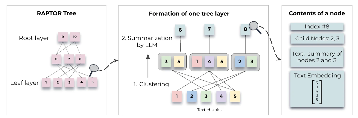
Three panels. Left: a RAPTOR tree with five leaf chunks at the bottom, three summary nodes above them, and two root nodes on top. Middle: one layer being built, where leaf chunks 1 to 5 are clustered into groups (3,5), (1,4,5) and (2,3), and each group is summarized by an LLM into nodes 6, 7 and 8; chunk 5 and chunk 3 each appear in two groups. Right: the contents of node 8, listing its index, its child nodes 2 and 3, a summary text, and a text embedding. — Figure 1 from Sarthi et al., 2024,⁶ reproduced under CC BY 4.0. Chunks are clustered by embedding, each cluster is summarized, and the process repeats upward.

At query time the paper's preferred method, the collapsed tree, ignores the layers and searches all nodes together, adding the best matches until it reaches 2,000 tokens.⁶ Summaries averaged 131 tokens and compressed their children by 72%.⁶ Across datasets and retrievers, 18.5% to 57% of the nodes it retrieved were summaries rather than leaves, so the upper layers were being used.⁶

In controlled runs with UnifiedQA-3B as the reader, adding the tree to SBERT raised QuALITY accuracy from 54.9% to 56.6% and QASPER F1 from 36.23 to 36.70.⁶ With GPT-4 on QASPER, RAPTOR scored 55.7 F1 against 53.0 for DPR.⁶ The headline number, 82.6% on QuALITY with GPT-4 against a previous best of 62.3%, compares against other published systems, not against the same reader with flat retrieval.⁶

Two details in the appendix are easy to miss. First, replacing the clustering with a plain tree that summarizes every 7 neighbouring chunks scored 55.8%, against 56.6% for the full method.⁶ My reading is that most of the gain comes from having summaries at all, and less from grouping chunks by meaning. Second, the per-story layer tables do not all favour the full tree. For one story, searching only the leaves scored 58.8 and searching all three layers scored 47.1.⁶ The summaries also cost accuracy at the source: in 150 hand-checked nodes, 4% contained minor hallucinations, which the authors found did not spread to parent nodes.⁶

What the papers could not measure

Nearly every study here scores chunks indirectly. Dense X Retrieval maps propositions back to passages, Bhat and colleagues use string matching, and Qu and colleagues map chunks to source documents or evidence sentences.^1,2,3 Qu, Bao and Tu say so directly in their limitations. There are no ground-truth relevance scores between queries and chunks, so different chunkers produced visibly different chunks but near-identical scores. Their stitched documents had artificially high topic diversity, and the sentence embeddings their semantic chunkers used carried no surrounding context. The authors write that "further exploration of contextual embeddings is necessary before definitively concluding the limitations of semantic chunking."³